Compliant ROS2 Controllers for Learning-Based Manipulation Policies

Daniel San José Pro

with Oliver Hausdörfer, Ralf Römer, Maximilian Dösch, Martin Schuck and Angela Schoellig

GitHub stars for utiasDSL/crisp_controllers

IEEE RAP 2026

learnsyslab.github.io/crisp_controllers

CRISP Controllers

Intro and overview

CRISP provides the low-level controller layer for learning-based manipulation.

1 Real-time controllers

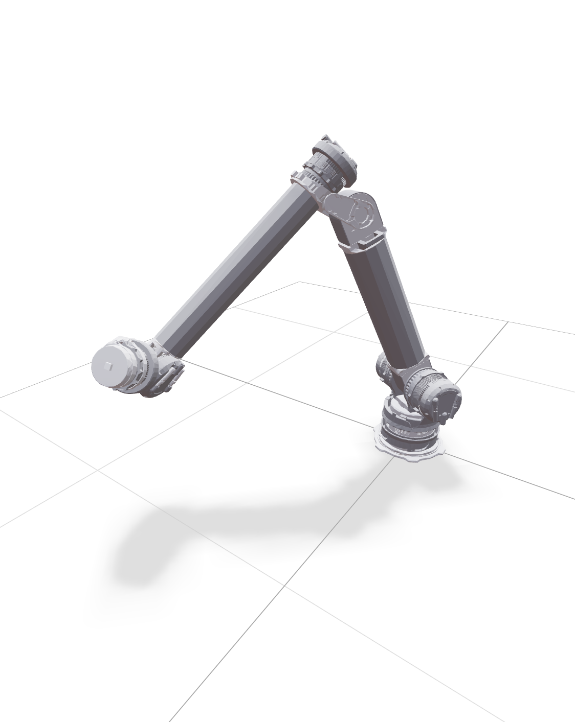
Compliant, robot-agnostic, torque-based ros2_control controllers running in real time on any manipulator with a joint-level effort interface.

2 One Python box

crisp_py and crisp_gym send target poses, joints, and wrenches, deploy Gymnasium and LeRobot policies, and collect synced episodes in LeRobotDataset format.

CRISP Controllers

Motivation · part 1

Stay smooth and compliant on sparse, low-frequency commands.

Franka Legocompliant pressing and stacking

Low-frequency input: sparse targets, poses, joints, or short action chunks.
High-frequency control: the controller closes the fast torque loop and keeps contact compliant.
No planning required: send simple commands and the controller fills in the rest.

CRISP Controllers

Motivation · part 2

The missing block: a controller that just tracks a stream of poses, compliantly.

The robot software stack

engineered modules

Sense

image_transport robot_localization

Plan

Nav2

Act

ros2_control

less code, more weights

Policy

absorbs perception + planningsparse pose targets · ~10 Hz

Controller

compliant · real-timethe CRISP block

CRISP Controllers

Joint control 101 · a starter

Drive a joint to a target angle with torque control

A stiffness gain Kp pulls the joint toward its goal angle.
A damping gain Kd settles the motion without overshoot.
Turn gravity on and the joint sags below its target: nothing in this law holds it up.
Task-space control next is the same idea, lifted into Cartesian space.

ττ
torque commanded to a single joint = K_pKp
joint stiffness gain: how hard the joint is pulled toward its target angle (q_desq_des
desired joint angle − qq
measured joint angle) − K_dKd
joint damping gain: resists joint velocity so the motion settles smoothly, without overshoot q̇q̇
joint velocity

QR code linking to the CRISP getting-started controller guide

more information ↗
learnsyslab.github.io/crisp_controllers · getting started

Kp closes the angle · Kd settles it

CRISP Controllers

Inverse dynamics 101

Turn end-effector forces in joint torques

Ask for a Cartesian force F.
Jᵀ maps that force into joint torques.

τ_cmdτcmd
joint torques sent to the robot = J^TJ
geometric Jacobian from joint motion to end-effector motion. Cartesian impedance uses it directly; operational-space control also folds in the task-space inertia Λ FF
desired end-effector force, chosen in the direction of the task-space error

Jᵀ / task-space force mapping: Khatib, “A unified approach for motion and force control of robot manipulators: the operational space formulation,” IEEE J. Robotics & Automation, 1987.

CRISP Controllers

CIC / OSC in one view

Turn cartesian space targets in proper joint torques

Cartesian controller

τ_tasktask torque
torque term that solves the Cartesian tracking task = J^TJ
geometric Jacobian. Cartesian impedance (CIC) uses it directly; operational-space control (OSC) folds in the task-space inertia matrix Λ. J can carry either. (K_pKp
stiffness gain in task space ee
pose error = X_target ⊖ X_current, the SE(3) difference between the desired and measured end-effector pose (translation and rotation handled separately) + K_dKd
damping gain in task space ėė
rate of the pose error. In practice this is the −end-effector velocity, which equals −J·q̇) e = X_target ⊖ X_current ė = −J q̇

e is the pose error: where the tip is versus where it should be.

Low stiffness

Less reactive, more compliant. Gentle, forgiving contact.

High stiffness

More reactive tracking, but larger forces and sharper accelerations against contact.

drag the target into the surface · toggle low / high stiffness

Impedance & stiffness: Hogan, “Impedance control,” ACC 1984. · CIC vs OSC: Nakanishi et al., “Operational space control: a theoretical and empirical comparison,” IJRR 2008.

CRISP Controllers

Same task, different posture

Keep the same end-effector goal, but ask for a better elbow configuration.

Add one more torque term to stabilize the joints positions

τ_cmdτcmd
final torque command = τ_taskτtask
task-space tracking torque + N(q)N(q)
nullspace projector that preserves the main end-effector task K_nsKns
nullspace posture gain ( q_targetq_target
preferred joint posture the arm is biased toward − qq
current joint state )

drag the target · purple ghost = target joint posture q_target

Null-space projections: Dietrich, Ott & Albu-Schäffer, “An overview of null space projections for redundant, torque-controlled robots,” IJRR 2015.

CRISP Controllers

Full controller synthesis

The deployed controller is a sum of torque terms, all fully parametrizable

Task tracking stays central. Around it we layer posture, model-based compensation, and interaction terms. A safety function then clamps the whole sum before it reaches the robot.

τ_cmdτcmd
final torque command sent to the robot = f_safetyf_safety
not another added term but a function over the whole sum. Clamps the total torque to the configured torque and rate limits before it reaches the robot τ_taskτtask
main Cartesian task-space tracking term + τ_nullτnull
the nullspace posture term from the previous slide, reused here unchanged + τ_jointτjoint
joint regularization, barriers, and limit handling + τ_modelτmodel
gravity, Coriolis, and friction compensation from the robot model + τ_wrenchτwrench
interaction or force-feedback term for teleoperation/contact

drag the target · layered terms keep tracking usable on real hardware

CRISP Controllers

Teleoperation with force feedback

The operator feels the contact the robot makes.

Feedback torque on the leader

τ_fbτfb
torque applied to the leader so the operator feels the follower's contact = −k_p,fbk_p,fb
force-feedback gain: how strongly follower contact is reflected to the leader J^TJᵀ
leader Jacobian, mapping the reflected Cartesian force into leader joint torques F_followerF_follower
contact force-torque measured at the follower's end-effector −k_d,fbk_d,fb
damping on the leader that keeps the coupled leader-follower loop stable q̇_leaderq̇_leader
leader joint velocity

Leader → follower

Pose streams over target_pose at ~30 Hz; the follower's CI controller does the tracking.

Follower → leader

The measured contact wrench is reflected as force feedback. Contact is felt, not guessed.

drag the leader arm (left) · the follower (right) tracks it and reflects contact force

Bilateral teleoperation: one of CRISP's three evaluation tasks: Lego block-stacking teleop with force feedback to the operator.

CRISP Controllers

Controller integration

The compliant controller plugs straight into the robot.

target_pose

target_joint

target_wrench

current_pose

current_joint

Policy

learned actions

Human

teleop, demos

crisp_py

crisp_gym

one interface: control + data

Recorder

logs from the same boundary

Controller

task-space torque

Broadcaster

publishes state + streams

Robot

hardware loop,
contact & sensing

commands

feedback

ros2_control plug

CRISP Controllers

One interface

crisp_py and crisp_gym are the shared interface for people, policies, and recording.

target_pose

target_joint

target_wrench

current_pose

current_joint

Policy

learned actions

Human

teleop, demos

crisp_py

crisp_gym

one interface: control + data

Recorder

logs from the same boundary

Controller

task-space torque

Broadcaster

publishes state + streams

Robot

hardware loop,
contact & sensing

commands

feedback

ros2_control plug

python · crisp_py

CRISP Controllers

Same interface, two recording philosophies

Collect synced episodes, or log everything and align it later.

target_pose

target_joint

target_wrench

Policy

learned actions

Human

teleop, demos

crisp_py

crisp_gym

one interface: control + data

LeRobotDataset

synced, training-ready

Timestamped data

e.g. MCAP, aligned later

Controller

task-space torque

Broadcaster

publishes state + streams

Robot

hardware loop,
contact & sensing

commands

feedback

ros2_control plug

Pros

No post-processing just to align sensors, actions, and targets.
Collection already matches training and deployment semantics.

Record any stream, tool, or debug signal you want.
Fits classic robotics logging with few constraints up front.

Cons

Less flexible than logging every stream in its own format.
You commit to the dataset structure earlier.

Alignment and shaping move to a later post-processing step.
Collection and training semantics drift apart more easily.

CRISP Controllers

What shipping changed

Open source in practice

Contributors

Across crisp_controllers, crisp_py, and crisp_gym.

DS

Daniel San José Pro@danielsanjosepro

OL

Oliver@OliEfr

ID

Ivan Domrachev@domrachev03

NM

Nabil Miri@Nabil-Miri

NI

niklasschlueter@niklasschlueter

DA

David Alexander@dmalexa5

VI

Vidullan@vidullan

VG

Veit Gemmer@veit1337

MD

Maximilian Dösch@maxdoesch

JS

Johannes Sautier@JohannesSautier

RR

Ralf Römer@ralfroemer99

LS

Linus Schwarz@Linus-Schwarz

LK

Lev Kozlov@lvjonok

LH

Luka Hofer@lukahofer

AL

AlexD@AlexD15216

BM

Bence Magyar@bmagyar

A lot happened after open-sourcing: new robots, PRs, Papers…

FR3 / Panda

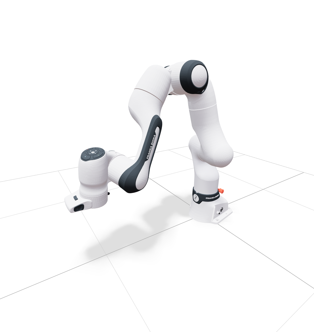
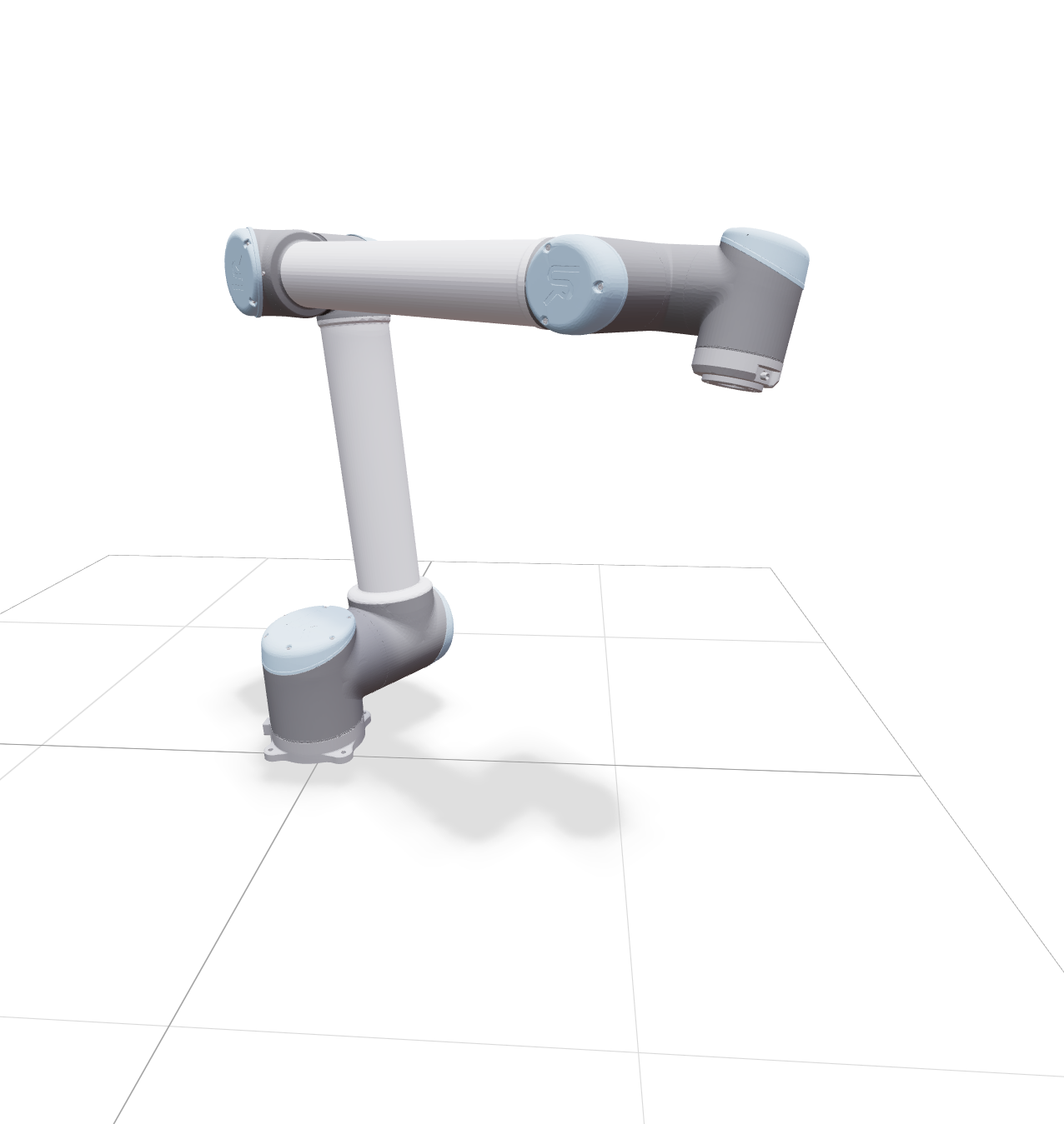
UR

DynaArm

Influential merged PRs

#46Variable Stiffness ControllerIvan Domrachev

#47Admittance ControllerIvan Domrachev

#57Decoupled admittance MSD integrationNabil Miri

#60Parameterize controller and broadcaster topicsDavid Alexander

Related work using CRISP

Failure prediction at runtime for generative robot policies
CLARE: Continual Learning for Vision-Language-Action Models via Autonomous Adapter Routing and Expansion
SQ-CBF: Signed Distance Functions for Numerically Stable Superquadric-Based Safety Filtering
From Demonstrations to Safe Deployment: Path-Consistent Safety Filtering for Diffusion Policies
Enabling Dynamic Tracking in Vision-Language-Action Models via Time-Discrete and Time-Continuous Velocity Feedforward

CRISP Controllers

General Learnings

Real-hardware evaluation is the bottleneckResets, supervision, timing bugs, and environment drift decide whether a success rate means anything.
Data collection is the controller problem tooCleaner demos and repeatable setup moved the Lego task from roughly 20% to 80% success.

CRISP Controllers

End of the tour

Thank you.
Questions?

Give it a try! Fork it, test it and share your deployments.

Scan for docs, install notes, and the repository.

learnsyslab.github.io/crisp_controllers

Compliant ROS2 Controllers for Learning-Based Manipulation Policies

CRISP provides the low-level controller layer for learning-based manipulation.

1 Real-time controllers

2 One Python box

Stay smooth and compliant on sparse, low-frequency commands.

The missing block: a controller that just tracks a stream of poses, compliantly.

Sense

Plan

Act

Policy

Controller

Drive a joint to a target angle with torque control

Turn end-effector forces in joint torques

Turn cartesian space targets in proper joint torques

Low stiffness

High stiffness

Keep the same end-effector goal, but ask for a better elbow configuration.

The deployed controller is a sum of torque terms, all fully parametrizable

The operator feels the contact the robot makes.

Leader → follower

Follower → leader

The compliant controller plugs straight into the robot.

Policy

Human

crisp_py

crisp_gym

Recorder

Controller

Broadcaster

Robot

crisp_py and crisp_gym are the shared interface for people, policies, and recording.

Policy

Human

crisp_py

crisp_gym

Recorder

Controller

Broadcaster

Robot

Collect synced episodes, or log everything and align it later.

Policy

Human

crisp_py

crisp_gym

LeRobotDataset

Timestamped data

Controller

Broadcaster

Robot

Pros

Cons

Open source in practice

Contributors

Influential merged PRs

Related work using CRISP

General Learnings

Thank you.Questions?

Thank you.
Questions?